Building a Simple Streaming Data Platform

Insights on streaming data are key in a number of industries — for example:

• Trading and fraud detection in finance
• Deriving insights about website traffic and social media engagement in online marketing
• Performing realtime price optimization and inventory management in retail
• Plus many other uses in these and other industries

Most data engineering tools are focused primarily on batch processing, leaving the streaming space as a smaller, but growing ecosystem.

I’m going to walk through an example of standing up core components of a streaming analytics platform including ingestion, data warehousing, observability, and an analytics tool. These provide some of the most visible components of a platform. In another article I’ll add on some of the key components for scaling and ongoing support of the platform.

If you’d like to follow along you can go to Github and grab the source code and configurations I use, along with detailed, but much more terse instruction on how to get everything working.

Ingestion

Before we can start performing analytics on our data, we need to get it into the system. In the world of batch data, we are spoiled for choice — Airbyte, Fivetran, Stitch, Meltano, and so on, each with a different set of tradeoffs. Most are quite straightforward to install and work with, to the point where they are useable by people with very limited technical depth.

In the streaming world our choices are more limited, though there are certainly good choices as well, such as Striim, Estuary, Databricks, Redpanda, Bento, and Flink. These solutions tend to be either proprietary or relatively complex. Due to the closed nature or complexity of the available solutions I’ve rolled my own for the purpose of this demo, with the goal of being simple and extensible rather than a full blown production solution, for which I would use one of the above. If you are interested in how I built ingestion you can find it here, under MIT license. The key takeaway is that it is easy to configure and run but lacks the delivery guarantees, backpressure handling, message configurability and resiliency of a production solution.

Data Warehouse

The next basic component of a data platform is a place to store the data. Again, in the world of batch-centric solutions we have many choices. In the streaming world, one key difference limits our available choices — the ability to handle ingestion of a large volume of data with low latency. I’m going to use Clickhouse since it is an incredibly fast data warehousing solution designed to handle streaming data well. It also handles batch data very effectively and is straightforward to work with at a small scale. Other possible choices would have been Druid, Pinot, Postgres with Timescale, or Databricks.

Installing Clickhouse

Assuming you have Docker installed (I’m using Docker Desktop on my MacBook), installing the container is by far the easiest option.

To start, just run:

docker pull clickhouse/clickhouse-server:latest 
docker run -d \ 
    --name clickhouse-server \ 
    -p 8123:8123 \ 
    -p 9000:9000

However, the danger of doing it this way is that none of the data is persisted to your local machine. When I run this, I tweak the above slightly:

docker run -d \ 
    --name clickhouse-server \ 
    --ulimit nofile=262144:262144 \ 
    -p 8123:8123 \ 
    -p 9000:9000 \ 
    -v $HOME/clickhouse/data:/var/lib/clickhouse \ 
    -v $HOME/clickhouse/config/clickhouse-server:/etc/clickhouse-server \ 
    -v $HOME/clickhouse/logs:/var/log/clickhouse-server \ 
    clickhouse/clickhouse-server:latest

It requires a bit more work as I must create the directories and configs, but it means that all of the config and data is stable.

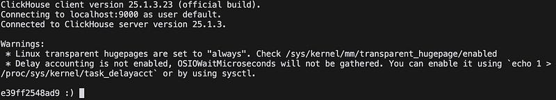
Once you’ve done this, you should have a Clickhouse server running locally. You can verify by running Clickhouse client:

docker exec -it clickhouse-server clickhouse-client

If you see the Clickhouse prompt, then your Clickhouse server is running and accessible.

In this prompt let’s create the database where we’ll store our data. I’m going to use the Coinbase trades feed since it is a freely available realtime feed with a moderate volume of data and enough differing feeds to make for interesting projects.

To create the database, run:

CREATE DATABASE IF NOT EXISTS coinbase_demo;

Now we’ll create the user we’ll be working with:

-- Create the user we'll be using in our tools to access Clickhouse 
CREATE USER coinbase IDENTIFIED BY 'password'; 
-- Grant permissions 
GRANT ALL ON coinbase_demo.* TO coinbase;

Finally, let’s create the table we’ll be using. In this case we’ll be storing tick data from a Coinbase trades feed.

-- Table for storing raw ticker data from Coinbase 
-- Note: Sorting key order (time, product_id, sequence) may not be optimal 
-- as time has higher cardinality than product_id, which is suboptimal 
-- for the generic exclusion algorithm 
CREATE TABLE IF NOT EXISTS coinbase_demo.coinbase_ticker  
( 
    sequence UInt64, 
    trade_id UInt64, 
    price Float64, 
    last_size Float64, 
    time DateTime, 
    product_id String, 
    side String, 
    open_24h Float64, 
    volume_24h Float64, 
    low_24h Float64, 
    high_24h Float64, 
    volume_30d Float64, 
    best_bid Float64, 
    best_bid_size Float64, 
    best_ask Float64, 
    best_ask_size Float64 
)  
ENGINE = MergeTree()  
ORDER BY (time, product_id, sequence);

Get Some Data

We’ve got our data store, so now let’s get some data into the system. I’m going to use the tool I built for this demo:

git clone https://github.com/Vertrix-ai/streaming-analytics-demo.git 
cd streaming-analytics-demo 
poetry install

In the root of the repo you’ll find a simple config for the tool. Make changes here if you have chosen to use a different database, username, etc.:

source: 
  wss_url: "wss://ws-feed.exchange.coinbase.com" 
  type: coinbase 
  subscription: 
    product_ids: 
      - "BTC-USD" 
    channels: 
      - "ticker" 
 
sink: 
  type: clickhouse_connect 
  host: "localhost" 
  port: 8123 
  database: "coinbase_demo" 
  table: "coinbase_ticker" 
  user: "coinbase" 
  password: "password"

Once you have that set you can start ingesting data:

poetry run python streaming_analytics_demo/listen.py --config demo_config.yaml

Give it a couple of seconds to make sure you have received messages and confirm that you now have data in Clickhouse:

select * from coinbase_demo.coinbase_ticker;

Observability

Before we start building analytics on our data we want to ensure that we trust the data we are receiving — without that, our analytics may produce bizarre results, or even worse, seemingly reasonable results that are wrong. We also want to make sure that our observability tools raise an alarm when there are issues. Otherwise, it is highly likely that no one will notice problems until it is too late.

As with ingestion and the data warehouse, the majority of the ‘Modern Data Stack’ tools are focused primarily on batch workloads. There are certainly tools that provide observability for streaming data, but they tend to be closed source. Since this is a demo, I’ll use open source tools to get a basic observability stack, based around Grafana. While Grafana is an unusual choice for a data stack, being more focused in the DevOps world, it provides the basic pieces we need.

We’ll start by building out a really basic measure — the rate at which we have been ingesting data per minute. We can (and should) look for other things as well, such as sequence gaps, trades for 0 volume, etc., but the rate is a good place to start, and the other measures have similar implementation.

We’ll start with just a query:

-- this query shows the number of rows ingested per minute 
 
-- CTE for each minute since the start of the data to now 
WITH time_series AS ( 
    SELECT  
        arrayJoin( 
            range( 
                toUnixTimestamp( 
                    (SELECT min(tumbleStart(time, toIntervalMinute(1))) 
                     FROM coinbase_demo.coinbase_ticker) 
                ), 
                toUnixTimestamp( 
                    (SELECT max(tumbleStart(now(), toIntervalMinute(1))) 
                     FROM coinbase_demo.coinbase_ticker) 
                ), 
                60  # increment by 60 seconds (1 minute) 
            ) 
        ) as minute 
), 
-- CTE to break out the trades by minute 
trade_by_minute AS ( 
    SELECT  
        tumbleStart(time, toIntervalMinute(1)) as minute, 
        time, 
        last_size, 
        product_id 
    FROM coinbase_demo.coinbase_ticker 
) 
-- select the minute and the number of rows ingested for each minute 
SELECT  
    fromUnixTimestamp(ts.minute) as minute, 
    countIf(t.last_size > 0 AND t.last_size IS NOT NULL) as num_rows 
FROM time_series ts 
LEFT JOIN trade_by_minute t ON fromUnixTimestamp(ts.minute) = t.minute 
GROUP BY ts.minute 
ORDER BY ts.minute DESC;

Running this query gives us a table showing the information we hoped for:

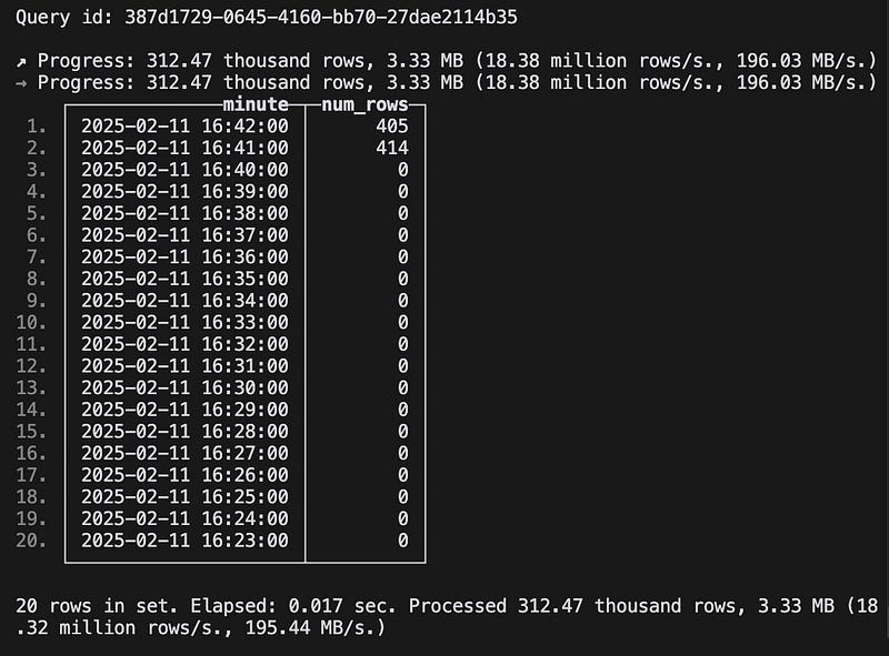
…but it isn’t very helpful. We can’t proactively alert on this, and people can’t see the results without manual steps that are both inefficient and unlikely to be done. An observability tool will make this information much easier to consume.

Installing Grafana

First, we’ll need to install Grafana which is available via Homebrew, so this is pretty straightforward:

brew update 
brew install grafana

Next is to get Grafana talking to Clickhouse. One of the advantages of having chosen relatively stable tools for this demo with broad adoption is that integrations are available.

Now we’ll install the Grafana Clickhouse plugin per their instructions. Let’s also create a read-only user for Grafana to access Clickhouse:

CREATE USER IF NOT EXISTS grafana IDENTIFIED WITH sha256_password BY 'password'; 
GRANT SELECT ON coinbase_demo.* TO grafana;

After this we’ll need to set up our configuration to allow Grafana to access Clickhouse. Grafana provides a way to configure plugins in the UI, but in the name of repeatability we’ll do it using a datasource config file:

apiVersion: 1 
datasources: 
  - name: ClickHouse 
    type: grafana-clickhouse-datasource 
    jsonData: 
      defaultDatabase: database 
      port: 9000 
      host: localhost 
      username: grafana 
      tlsSkipVerify: false 
    secureJsonData: 
      password: password

Now we can place the config file in the grafana provisioning directory and restart Grafana:

cp ~/projects/streaming_analytics_demo/observability/datasource.yaml provisioning/datasources/ 
brew services restart grafana

Now that we have all of this set up, go to http://localhost:3000 and log in. The default credentials are ‘admin/admin’ which you will be asked to change after login.

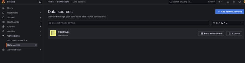
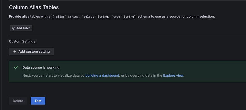
Go to connections->data sources and you should see the Clickhouse datasource. Scroll down to the bottom and click the ‘Test’ button. You should see a message that says ‘Data source is working’.

Observability Dashboard

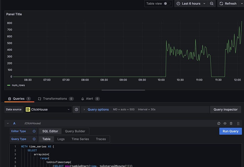
Now that we have Grafana installed and connecting to Clickhouse we want to build a dashboard for the query we built above.

In the menu, click on ‘Dashboards’. Click on ‘New’ and then ‘Add visualization’. Select the Clickhouse datasource and ‘SQL Editor’. Run the rows ingested per minute from above and you’ll see a graph of the ingestion rate. Click ‘Save’ and give your dashboard a name.

Observability isn’t just about graphing — we can also use the data to trigger alerts, so let’s add an alert to our dashboard. Click on the ‘Alerting’ tab and then ‘New Alert Rule’.

From here we’ll add a new query:

-- Query to ensure we have received ticks in the last minute 
SELECT 
    count(sequence) 
FROM coinbase_ticker 
WHERE time > now() - INTERVAL 1 minute;

In the ‘options’ we’ll set this to run every minute.

We’ll then add a new ‘Threshold’ on Input ‘A’ and set the condition to ‘Is Below’ 1. As long as you have run your query and see that messages have been received in the last minute, you should see that the alert condition is ‘normal’. Now you can save the alert and exit. You should see the alert in the ‘Alert rules’. There’s also an option to set up email notifications if you so choose.

Now, stop the ingestion and you will see your Alert rule change to ‘firing’. You can also see that the incoming messages have stopped on your dashboard. Restart the ingestion and watch the alert return to ‘normal’. This also illustrates the importance of monitoring your data. If we hadn’t been monitoring, we wouldn’t have known that the ingestion had stopped until we got some strange results from our analytics — which may have been too late. There is a lot more that can be done here, but this provides a good starting point.

Improvements

One of the things you’ll immediately notice is that in our dashboard we are running a query every minute to refresh the data. Taking a look at the query, on what for Clickhouse is quite a small dataset, gives the following timing information on my laptop:

5304 rows in set. Elapsed: 0.046 sec. Processed 791.55 thousand rows, 8.44 MB (17.23 million rows/s., 183.77 MB/s.) 
Peak memory usage: 37.01 MiB.

Running that query every minute is a waste of resources. We can do better by using a materialized view.

First, in the Clickhouse client, create a table to store the trades per minute.

-- Table to store the number of trades per minute 
-- Uses SummingMergeTree to efficiently handle updates to the num_trades 
CREATE TABLE IF NOT EXISTS coinbase_demo.trades_per_minute 
( 
    minute DateTime, 
    num_trades UInt64 
)  
ENGINE = SummingMergeTree() 
ORDER BY minute;

Notice the use of ‘SummingMergeTree()’ This is a special engine for summing sequential data. As new data is ingested it is summed up at merge time, maintaining fast inserts but removing the need to sum all rows each time we query the table.

We then create a materialized view that updates the trades per minute table:

CREATE MATERIALIZED VIEW IF NOT EXISTS coinbase_demo.trades_per_minute_mv 
TO coinbase_demo.trades_per_minute 
AS 
SELECT  
    tumbleStart(time, toIntervalMinute(1)) as minute, 
    countIf(last_size > 0) as num_trades 
FROM coinbase_demo.coinbase_ticker 
GROUP BY minute;

Notice the ‘TO’ keyword here. This is how we tell the materialized view to update the trades per minute table. The select statement gives the query to source the incoming data, in this case the Coinbase ticker table where the raw data is stored.

Now we’ll run the old query against a table where I’ve had ingestion running for a while. We are processing 916.94 thousand rows — the entire table — which would not scale terribly well.

5819 rows in set. Elapsed: 0.025 sec. Processed 916.94 thousand rows, 9.78 MB (36.19 million rows/s., 386.05 MB/s.) 
Peak memory usage: 37.02 MiB.

Now let’s run a new query that uses the materialized view and produces the same result:

WITH time_series AS ( 
SELECT  
    arrayJoin( 
        range( 
            toUnixTimestamp( 
                (SELECT min(minute) 
                 FROM coinbase_demo.trades_per_minute) 
            ), 
            toUnixTimestamp( 
                (SELECT tumbleStart(now(), toIntervalMinute(1))) 
            ), 
            60  -- increment by 60 seconds (1 minute) 
        ) 
    ) as minute, 
    0 as num_trades 
), 
-- We need to get the sum of the trades per minute because the  
-- SummingMergeTree delays the summing until merge time. This is  
-- done for insert performance, so the most recent minute may have 
-- not been summed yet. 
summed_trades AS ( 
    SELECT  
        minute, 
        sum(num_trades) as num_trades 
    FROM coinbase_demo.trades_per_minute 
    GROUP BY minute 
    ORDER BY minute DESC 
), 
-- Now we join the time series with the summed trades to get the trades 
-- per minute. 
SELECT  
    fromUnixTimestamp(ts.minute) as minute, 
    greatest(ts.num_trades, t.num_trades) as num_trades 
FROM time_series ts 
LEFT JOIN coinbase_demo.trades_per_minute t ON fromUnixTimestamp(ts.minute) = t.minute 
ORDER BY minute DESC;

This new query is much more efficient. It processes only the 5834 rows that are currently found in the trades_per_minute table. While both queries return very quickly on this dataset, the difference will become more pronounced as the dataset grows.

5834 rows in set. Elapsed: 0.026 sec.

We can go back to our dashboard and replace the old query with the new one.

Analytics Tooling

Now that we have some data in our database and the ability to detect problems with it, let’s look at performing some analytics. Looking at the tools we have, you could argue that we already have what we need — after all, we can run queries in Grafana and create dashboards based on that. The issue is that Grafana is really targeted at observability and time series monitoring. It is designed to be easy for infrastructure teams to work with and does not have the rich user experience and support for ad hoc analysis that can be found in other tools. So let’s integrate a purpose-built BI tool by installing Superset.

Installation

I’m going to use Docker Compose to install Superset for this demo. This is not a production-grade installation, but it is easy for demo purposes. To start with we’ll need to clone the Superset repo:

git clone - depth=1 https://github.com/apache/superset.git 
cd superset

Before we start the container, we’ll need to install the dependencies and make some configuration changes:

touch ./docker/requirements-local.txt

Edit your new requirements-local.txt file to include the following:

clickhouse-connect>=0.6.8

Now we can start Superset:

docker compose -f docker-compose-non-dev.yml up

This one is going to take a while to start up. It’s downloading all the dependencies and building the Superset image. Once it has finished you should be able to access the Superset UI at http://localhost:8088. Unless you’ve changed the admin password you can use admin/admin to login. From here click on the ‘+’ on the top right, and select Data -> Connect Database.

If you’ve succeeded in adding Clickhouse then it will be available in the ‘supported databases’.

Analytics

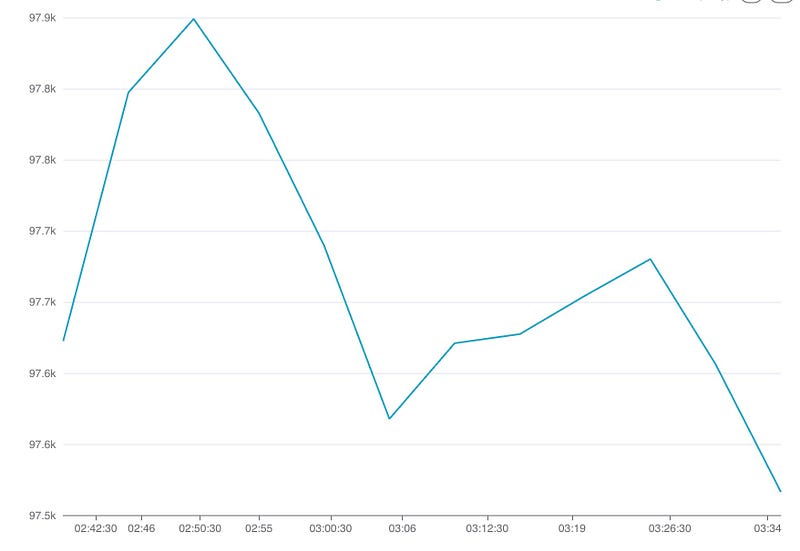
Now that we have the infrastructure in place, let’s perform our analytics. We’re looking at a trading dataset, so let’s build out a dashboard showing the 5 minute Volume Weighted Average Price (VWAP) for the last 24 hours.

The first step is to add a Superset dataset with our tick data. Superset provides multiple ways to do this — we can create a dataset from a table in our database and create a chart from that using a builder, or we can use the SQL Lab to write a query and then build a chart from that. I’ll take the latter approach.

Let’s navigate to the SQL Lab and build our query:

-- Construct a series of 5 minute periods for the prior 24 hours 
-- which is the period we want to chart 
WITH time_series AS ( 
    SELECT  
        arrayJoin( 
            range( 
                toUnixTimestamp( 
                    (SELECT tumbleStart((now() - INTERVAL 24 HOUR), toIntervalMinute(5))) 
                ), 
                toUnixTimestamp( 
                    (SELECT tumbleStart(now(), toIntervalMinute(5))) 
                ), 
                300  -- increment by 300 seconds (5 minutes) 
            ) 
        ) as interval 
), 
-- Calculate the components of the vwap 
vwap AS ( 
    SELECT  
        tumbleStart(time, toIntervalMinute(5)) as period, 
        SUM(price * last_size) as volume_price, 
        SUM(last_size) as total_volume 
    FROM coinbase_demo.coinbase_ticker 
    WHERE  
        period >= now() - INTERVAL 24 HOUR 
        AND last_size > 0  -- Filter out zero volume trades 
        AND price > 0      -- Filter out invalid prices 
    GROUP BY period 
) 
-- Join the vwap calculation to the time series to give the 5 minute vwap for the last 24 hours 
SELECT  
    fromUnixTimestamp(interval) as vwap_period, 
    IF(v.total_volume > 0, v.volume_price/v.total_volume, 0) as vwap 
FROM time_series ts 
LEFT JOIN vwap v ON fromUnixTimestamp(ts.interval) = v.period 
ORDER BY vwap_period DESC;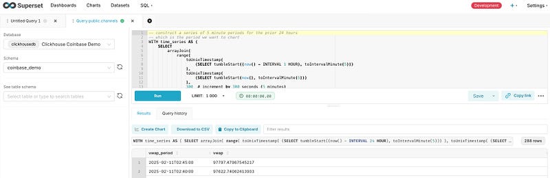

To build the chart, select the chart button below the query and then fill out the wizard like this:

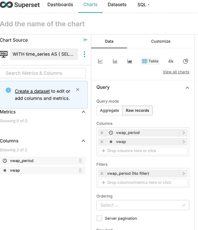
You can now save the chart, at which point you will be asked which dashboard you’d like to add it to.

Finally, we can edit the dashboard by clicking on the ‘…’ and set a refresh interval for the dashboard. That will give us a dashboard updating every 10 seconds.

The same performance concerns we had with ingestion monitoring apply here; Superset is just rerunning the full query every time. I won’t go into how to create the materialized view again — it is the same process we used before.

Conclusion

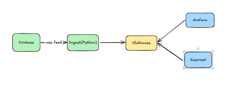
At this point we have data ingestion via a custom python tool, a highly performant data warehouse in Clickhouse, observability via Grafana, and analytics via Superset. We’ve seen how we can store and query streaming data in Clickhouse, use materialized views to offload some of our compute from query time to load time, and present useable tools for analytics and monitoring.

We’ve delivered value for the end users of the platform — but we’re not done. This will hold up well initially, but inevitably on the business side we’ll run into questions about what the data means as the number of datasets grows, the lineage of our data, and what assertions we can make about its quality.

On the engineering side we also still have work to do. The system implements baseline functionality, but as we scale we’ll run into problems managing it if we leave it in this state. We’ve started writing some interesting queries, and the source of truth for our data models and our transformations is split between the database and our BI tool. We’ll run into problems where we break queries, where we have trouble tracking down how datasets are derived, and will very likely cause ourselves production issues as we make changes. We’ll look at how we can address these issues in the next post.

Have you set up a streaming data platform? What tech stack did you choose and why? Would love to hear in the comments.